Homography Estimation and Image Stitching

GitHub

Overview

This project demonstrates the creation of a seamless panoramic image from a set of 5 images captured by roating the camera at one place and refining the Homography estimation between them fro image stiching task. The process leverages robust feature detection, matching, homography estimation with RANSAC, and final image stitching with blending techniques to minimize seams.

Pipeline Details

1. Image Preprocessing

• Grayscale Conversion: All images are converted to grayscale to simplify processing.
• Corner Detection: The Harris corner detection algorithm is applied to identify prominent corner features.
• Corner Response Calculation: The Harris R function quantifies the strength of detected corners.

2. Feature Matching

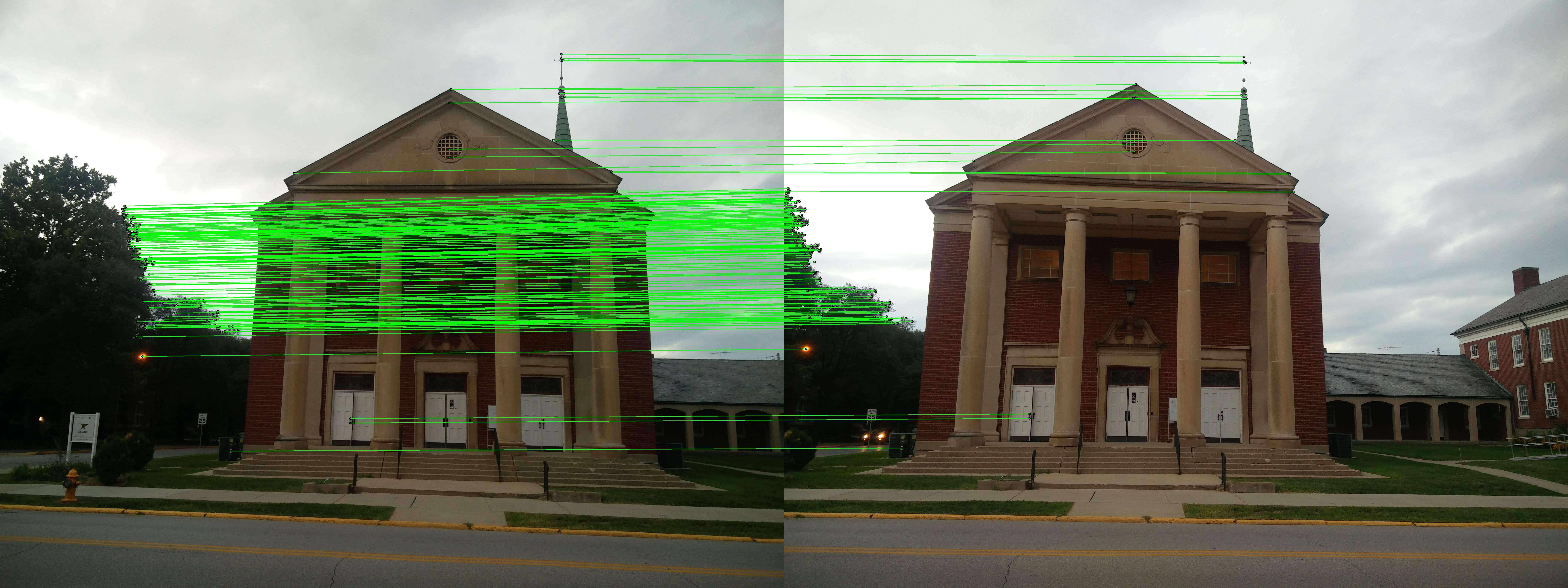
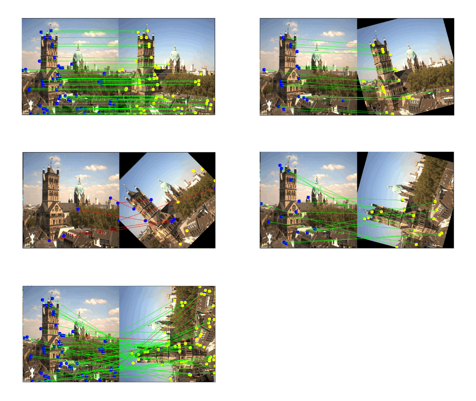
• Descriptor Extraction: Feature descriptors are extracted from the detected corner points.

• Normalized Cross Correlation (NCC):
  Correspondences between images are established using NCC, defined as after getting the correspondence we need to filter out the wrong correspondences such as outlier:

  \[NCC = \frac{\sum_{i=1}^{25} x(i) \, y(i)}{\sqrt{\left(\sum_{i=1}^{25} x(i)^2\right) \left(\sum_{i=1}^{25} y(i)^2\right)}}\]

3. Homography Estimation with RANSAC

• Random Sampling:
  A minimal set of 4 matching points is randomly selected to compute a candidate homography matrix ( H ).

• Inlier/Outlier Filtering:
  For each candidate homography, the reprojection error for a correspondence is computed as:

  \[e_i = \left\| \mathbf{x}'_i - H\,\mathbf{x}_i \right\|\]

  A correspondence is classified as an inlier if \((e_i < \epsilon \), where ( \epsilon \)\) is a predetermined error threshold. The inlier count is given by:

  \[\text{inlier\_count} = \sum_{i=1}^{N} \mathbb{I}(e_i < \epsilon)\]

  Here, ( \mathbb{I}(\cdot) ) is the indicator function that returns 1 if the condition is met, and 0 otherwise.

• Iteration and Model Selection:
  RANSAC iterates to find the best homography. The number of iterations ( k ) required to achieve a desired probability ( p ) of selecting an outlier-free subset (given an outlier ratio ( \delta ) and a sample size ( n )) is estimated by:

  \[k = \frac{\log(1-p)}{\log\left(1-(1-\delta)^n\right)}\]

  The candidate homography with the highest inlier count is chosen for further processing.

4. Image Rectification, Stitching, and Blending

• Warping:
  Each image is warped into a common coordinate frame using the estimated homography matrices.genrally i took the 3 or the middle image in the sample to be my first image and calculated homgrahy in both the sides and then warped them to the persepctive of the miidle image stcing from both sides

• Stitching:
  The warped images are stitched together to form a continuous panorama.

• Blending:
  Overlapping regions are blended using techniques that smooth transitions and minimize visible seams, resulting in a cohesive final image. there are many blending techniques that can be used to blend image like - Alpha blending , Weighted avergae blending Etc

5. Constructing the Panorama from 5 Images

• Feature Matching and RANSAC Filtering:
  Feature correspondences between each adjacent pair of images are established, and RANSAC is used to determine inliers, discarding outliers to accurately estimate the homography matrix.
• Homography Estimation and Image Rectification:
  Using the inlier set, the homography matrix is computed for each image pair, and images are rectified accordingly.
• Final Stitching and Blending:
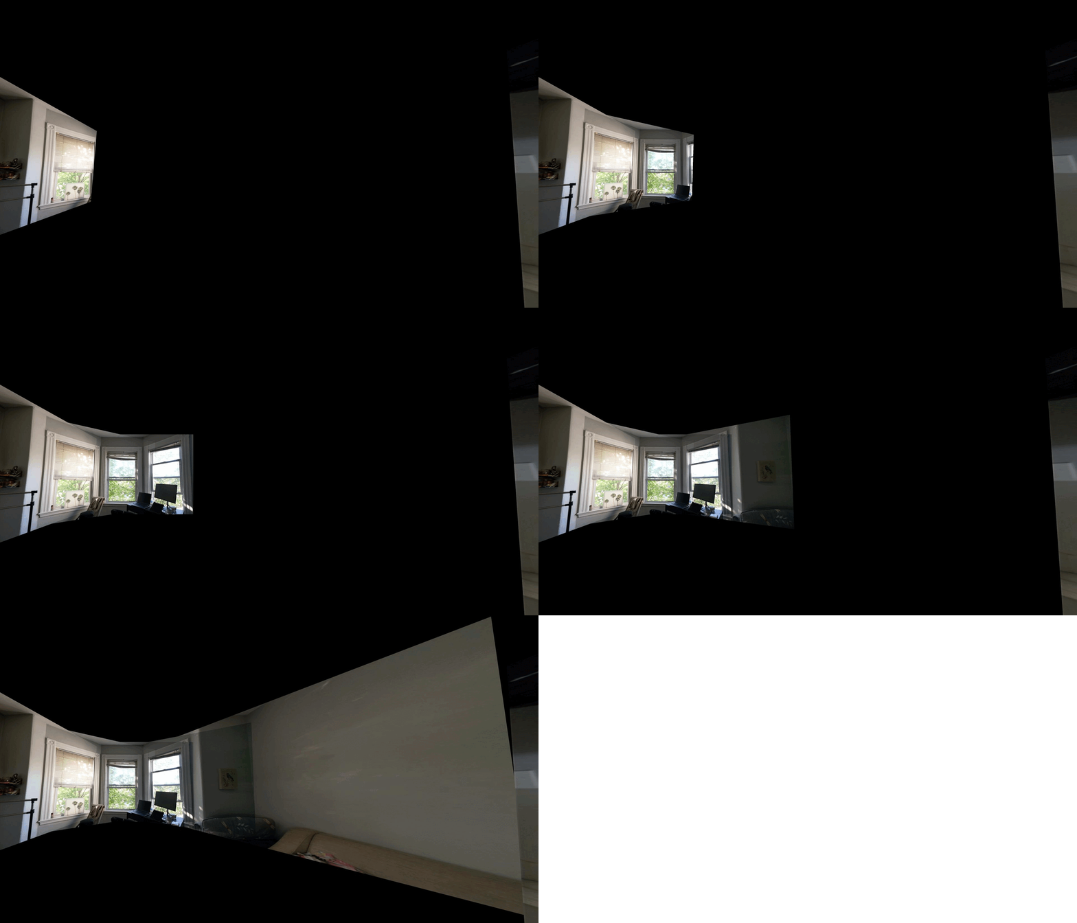
  The rectified images are then stitched together in sequence. Advanced blending techniques ensure a smooth transition across image boundaries.

Homography Matrix

For any two images of the same planar scene, the mapping between corresponding pixel coordinates is given by the homography matrix:

Here, ( (lx’, ly’) ) are the coordinates in the left image and ( (rx, ry) ) are the corresponding coordinates in the right image.

Visual Results After RANSAC Filtering

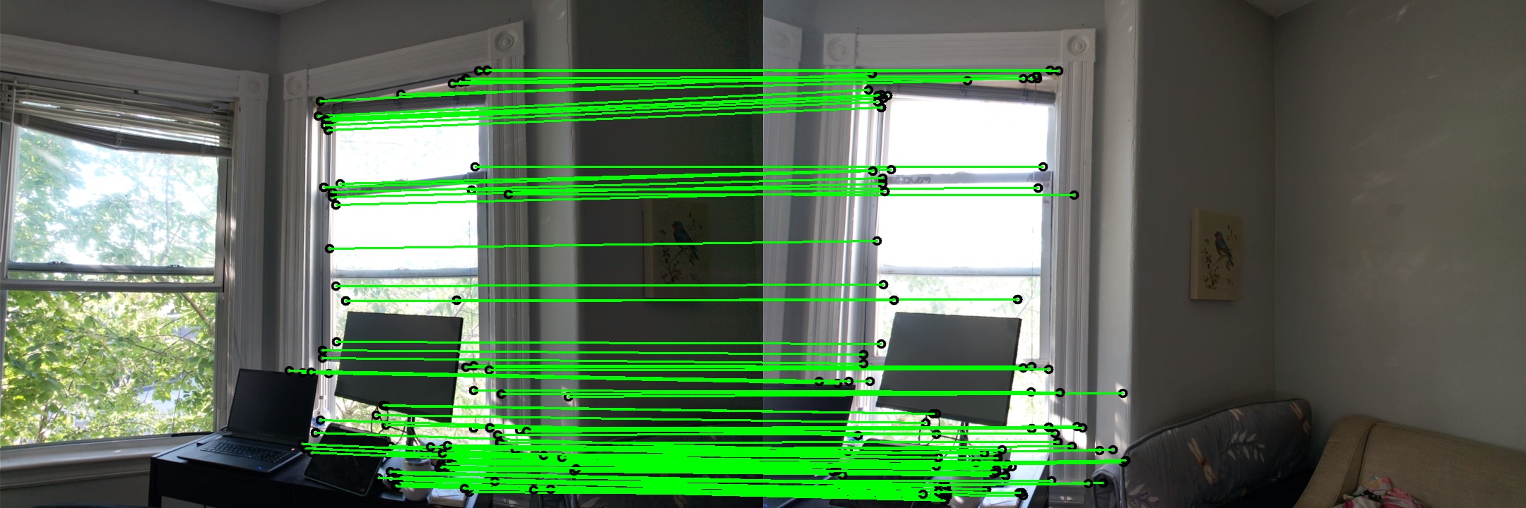
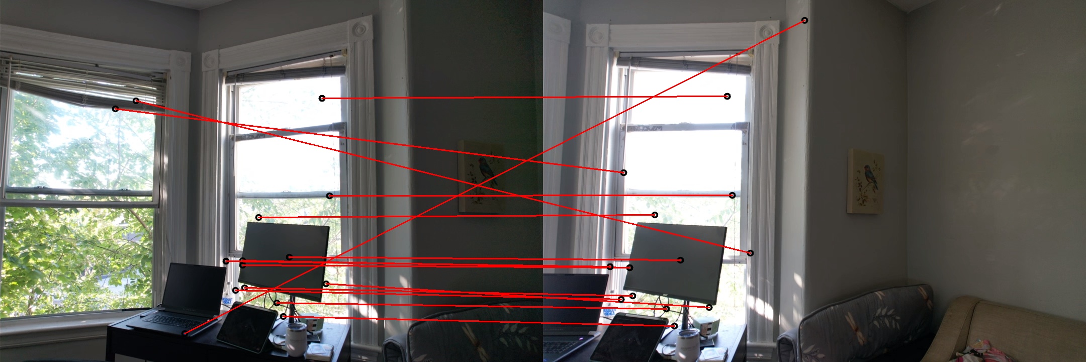
These images display the feature matching results before and after applying RANSAC. The left image shows the inliers (correct matches), while the right image displays the outliers (incorrect matches):

Dataset 2

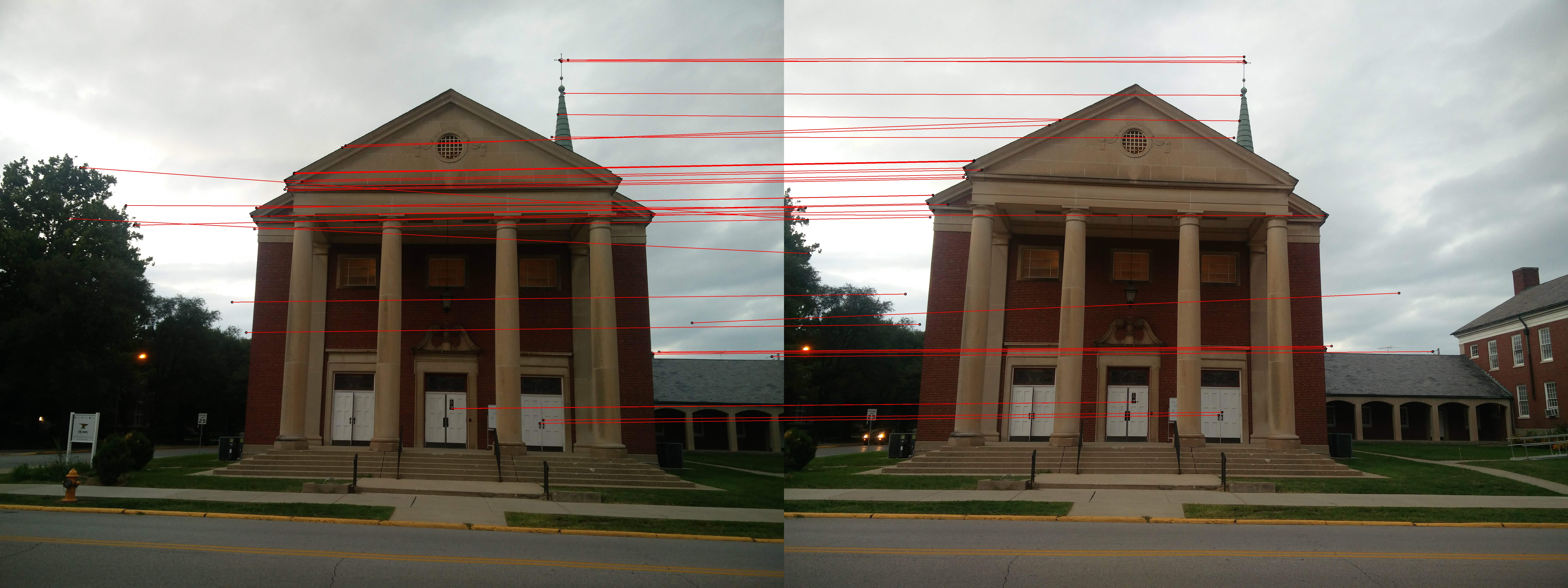
Image Set for Panorama Stitching

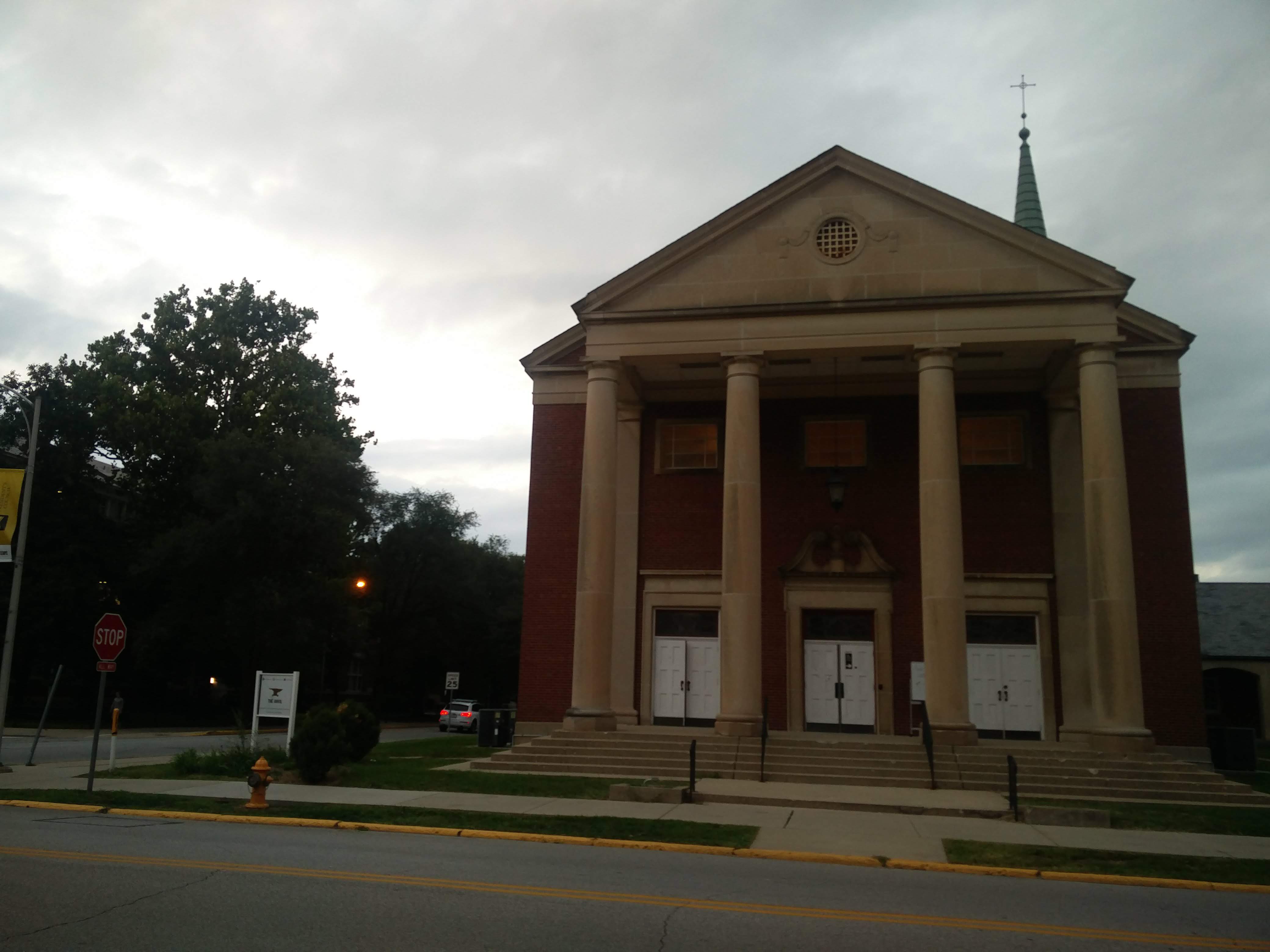
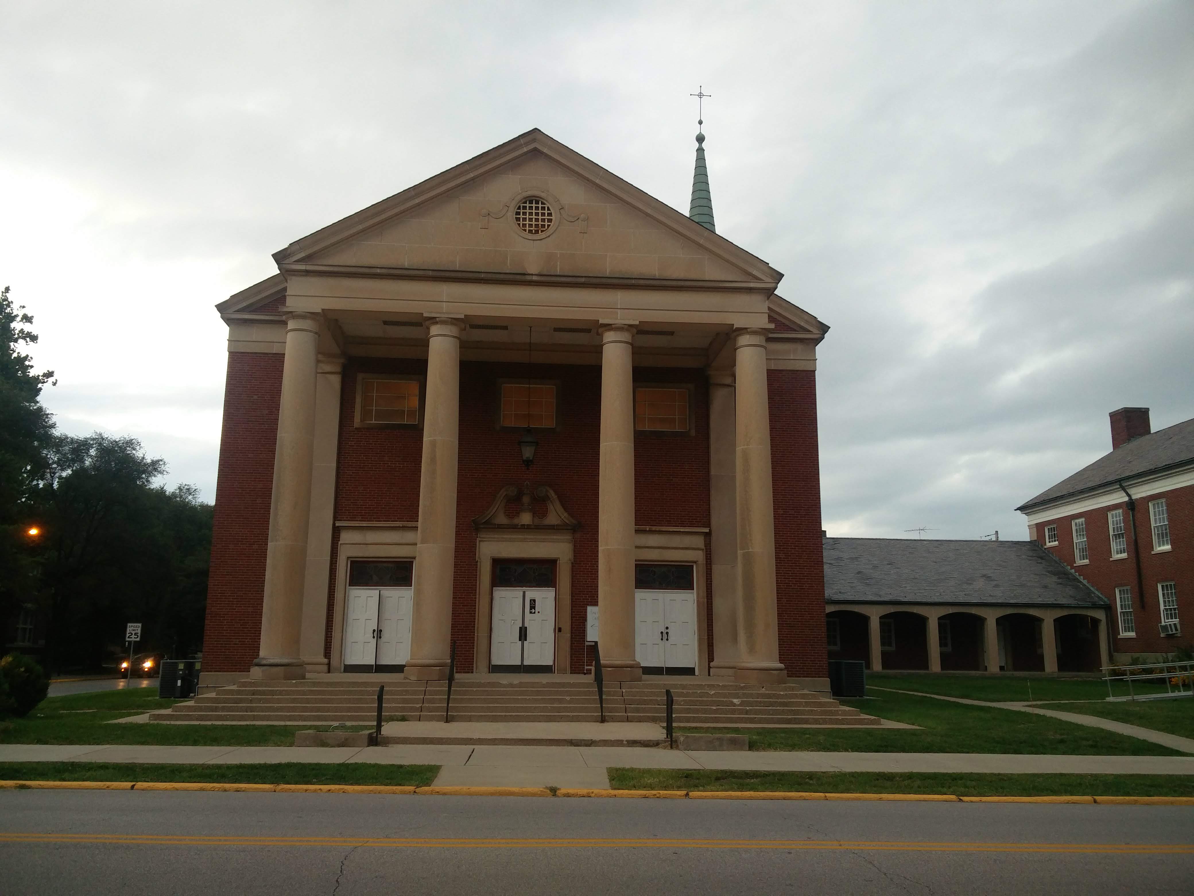
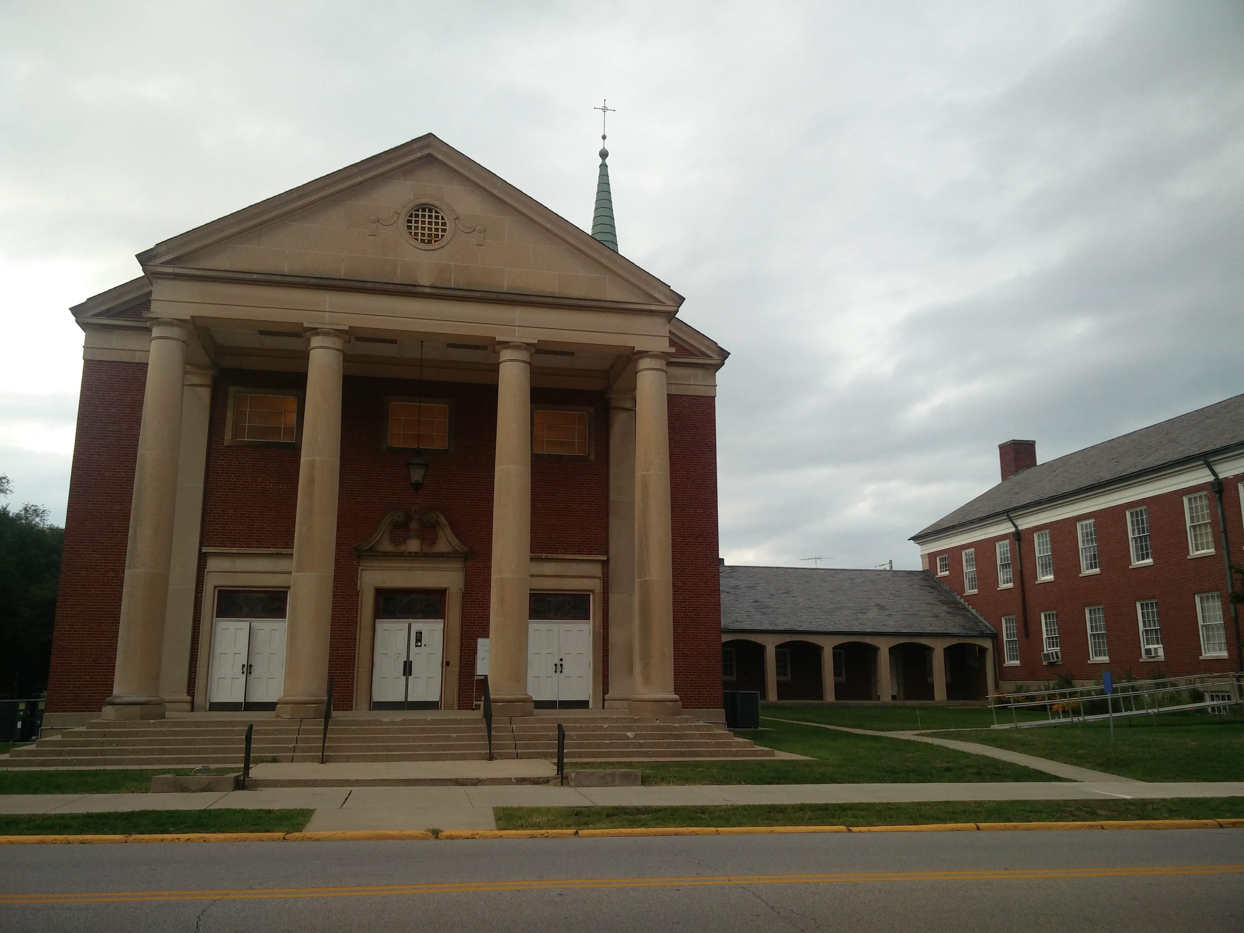
The following set of images were used to construct the final panorama:

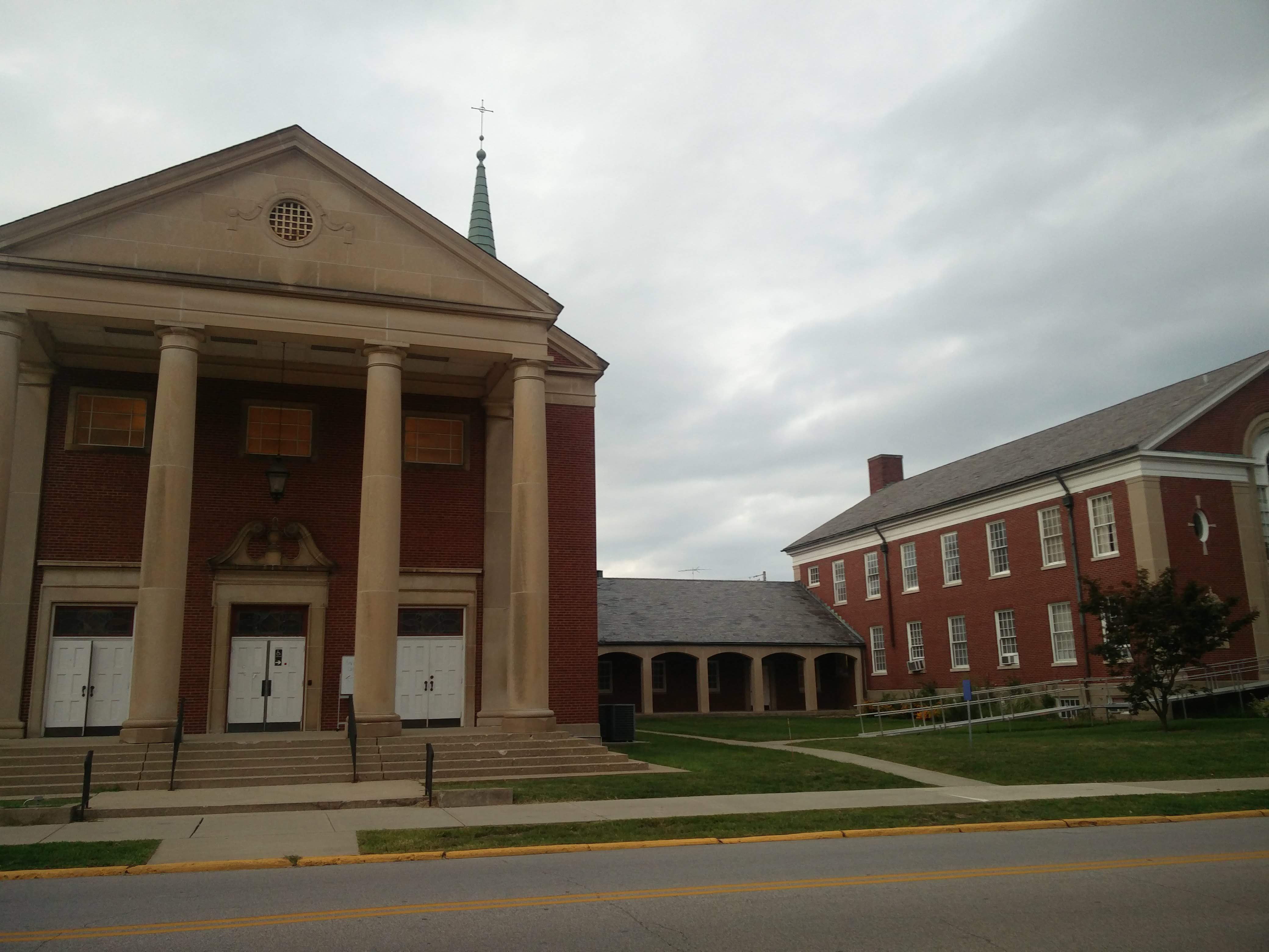
Additional Church Image Set

Final Mosaic Results

The final panoramas after stitching and blending:

Conclusion

By integrating feature matching, RANSAC-based homography estimation, and careful stitching with blending techniques, this pipeline successfully constructs a panoramic view from a set of 5 underwater images. This robust approach addresses challenges such as low lighting and image distortions, paving the way for further enhancements in underwater image mosaicing.